Back in 2017, I used to tease my friend about his machine learning work (training models, dataset operations, ML deployments) - “Come on, admit it, aren’t you just writing complex if-elif-else statements and calling yourself an ML engineer?”. While Google was bringing ML models to mobile devices using tensorflow, I remained indifferent as I couldn’t grasp the underlying mathematics or internal workings (which, honestly, continues to this day).
 {:height=“400px”}
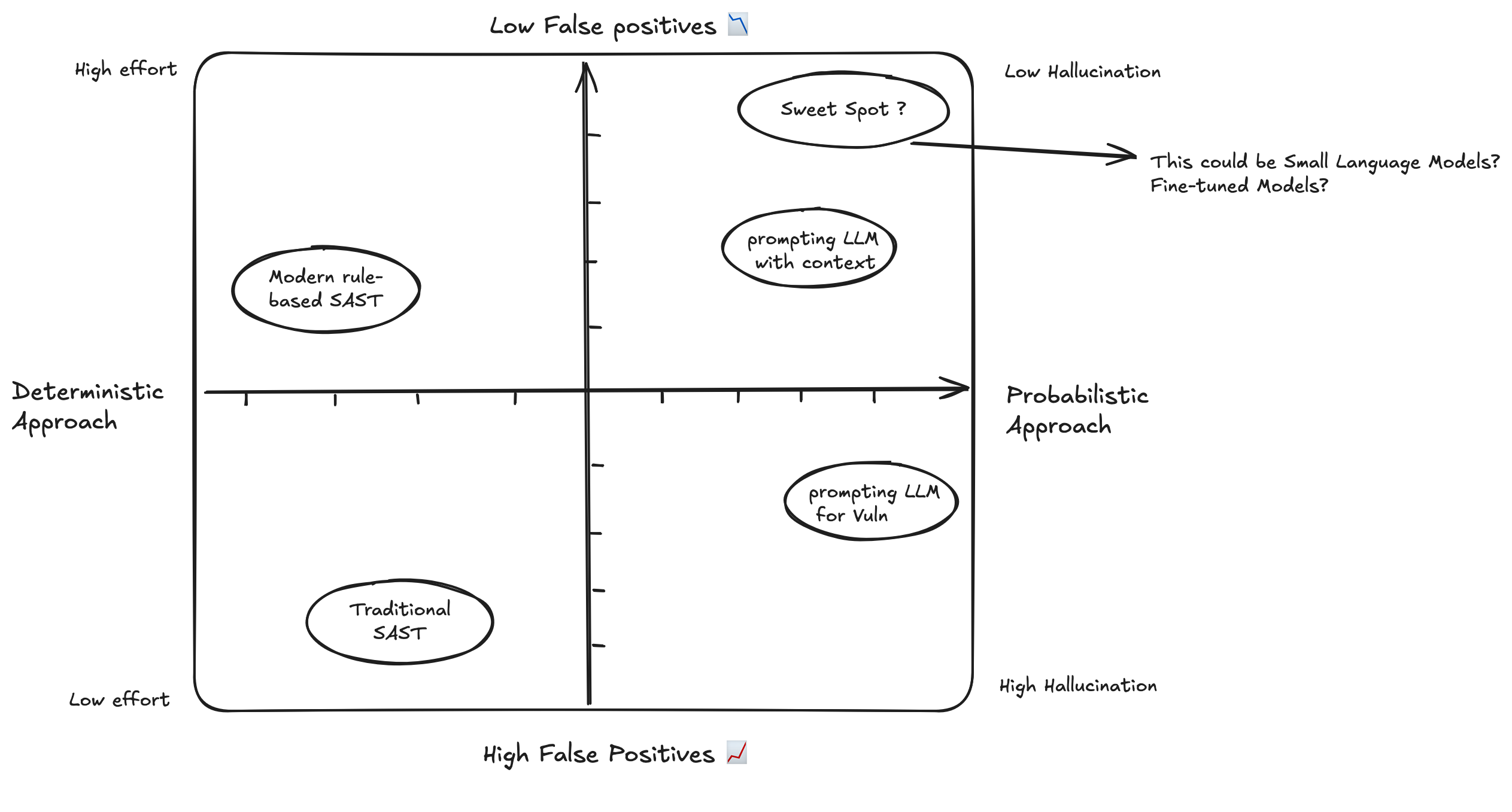
My perspective shifted after diving deep into projects like Sherlock, LLM-Powered Security Reviews, and SecureFlow AI. After studying numerous research papers about using language models to detect code vulnerabilities, I felt compelled to return to the basics and understand the fundamental workings of neural networks, particularly how they store information in their hidden layers.
This got me thinking - if large language models are capable of detecting these vulnerabilities, couldn’t a well-trained smaller model accomplish similar tasks? Perhaps with lower accuracy, but still useful? While I acknowledge my limited expertise in model scaling and benchmarking, the question intrigued me enough to explore the fundamentals of neural networks and understand their capabilities at different scales.
Driven by curiosity to understand the hidden layer mechanics (thanks to 3Blue1Brown’s excellent explanations), I implemented a basic neural network for the XOR operation. Interestingly, while this example uses the sigmoid activation function, modern networks typically prefer ReLU for better performance and to avoid vanishing gradient problems.
Building a small XOR neural-net 🤯
I got mind-blown after running this “hello world” example and watching 3Blue1Brown’s explanation. It helped me grasp the fundamentals in a way I hadn’t before. Some might question why we’d bother training a neural network for XOR when we could simply use the operator directly. However, the fascinating part isn’t the XOR operation itself, but how neurons learn and store weights based on input patterns to generate accurate outputs.
The real power lies in how this concept scales. Instead of writing explicit logic for each operation, the network learns patterns from training data and can make predictions efficiently. Think of it like a smart lookup table - rather than programming every possible case, we train the network once and can run inference countless times. While this might seem overkill for XOR, the same principles apply to much more complex problems where traditional programming approaches would be impractical.
# train.py
import numpy as np

# Sigmoid activation function and its derivative
def sigmoid(x):
    return 1 / (1 + np.exp(-x))

def sigmoid_derivative(x):
    return x * (1 - x)

# --- Dataset ---
X = np.array([[0, 0], [0, 1], [1, 0], [1, 1]])
y = np.array([[0], [1], [1], [0]])

# --- Network Architecture ---
input_neurons = 2
hidden_neurons = 4
output_neurons = 1
learning_rate = 0.1

# --- Initialize Weights ---
# Use a seed for reproducibility
np.random.seed(42)
weights0 = np.random.uniform(size=(input_neurons, hidden_neurons))
weights1 = np.random.uniform(size=(hidden_neurons, output_neurons))

print("Starting training...")

# --- Training Loop ---
for epoch in range(10000):
    # Forward Propagation
    hidden_layer_input = np.dot(X, weights0)
    hidden_layer_output = sigmoid(hidden_layer_input)
    output_layer_input = np.dot(hidden_layer_output, weights1)
    predicted_output = sigmoid(output_layer_input)

    # Backpropagation
    error = y - predicted_output
    d_predicted_output = error * sigmoid_derivative(predicted_output)

    error_hidden_layer = d_predicted_output.dot(weights1.T)
    d_hidden_layer = error_hidden_layer * sigmoid_derivative(hidden_layer_output)

    # Update Weights
    weights1 += hidden_layer_output.T.dot(d_predicted_output) * learning_rate
    weights0 += X.T.dot(d_hidden_layer) * learning_rate

# --- Save Trained Weights ---
np.save('weights0.npy', weights0)
np.save('weights1.npy', weights1)

print("Training complete. Weights have been saved.")
print("\nFinal output after training:")
print(predicted_output)
Output
(.venv) shiva@shivasurya ~/src/shivasurya/xor_project python3 train.py
Starting training...
Training complete. Weights have been saved.
Final output after training:
[[0.10125271]
[0.92688325]
[0.92005246]
[0.05933504]]
(.venv) shiva@shivasurya ~/src/shivasurya/xor_project python3 inference.py
enter left operand
1
enter right operand
1
Input: [1 1]
Raw Prediction Output: 0.0593
Final Prediction (1 XOR 1): 0
I progressed to more advanced examples like the MNIST digits classification (reminiscent of Yann LeCun’s 1989 Demo). This experience sparked my interest in exploring sophisticated models like BERT and fine-tuning with custom datasets, focusing on inference using desktop CPU/laptop GPU rather than extensive GPU clusters required for large language models.
Closing Note
This post reflects my ongoing journey of exploring how LLMs can revolutionize security reviews and vulnerability hunting. While there are still challenges to overcome, the potential is undeniable. I hope you find this blog post useful. For bugs or hugs & discussion, DM me on X. Opinions are my own and not the views of my employer.